PyTorch

Environment setup

import platform

print(f"Python version: {platform.python_version()}")
assert platform.python_version_tuple() >= ("3", "6")

import numpy as np
import matplotlib
import matplotlib.pyplot as plt
import seaborn as sns

Python version: 3.7.5

# Setup plots
%matplotlib inline
plt.rcParams["figure.figsize"] = 10, 8
%config InlineBackend.figure_format = 'retina'
sns.set()
%load_ext tensorboard

import sklearn

print(f"scikit-learn version: {sklearn.__version__}")

from sklearn.datasets import make_moons

import torch

print(f"PyTorch version: {torch.__version__}")

import torch.nn as nn
import torch.nn.functional as F
import torch.optim as optim
import torchvision
import torchvision.transforms as transforms
from torch.utils.tensorboard import SummaryWriter

scikit-learn version: 0.22.1
PyTorch version: 1.3.1

Show code cell source Hide code cell source

def plot_planar_data(X, y):
    """Plot some 2D data"""

    plt.figure()
    plt.plot(X[y == 0, 0], X[y == 0, 1], 'or', alpha=0.5, label=0)
    plt.plot(X[y == 1, 0], X[y == 1, 1], 'ob', alpha=0.5, label=1)
    plt.legend()

Tensor API

Tensor creation

# Create 1D tensor with predefined values
t = torch.tensor([5.5, 3])

print(t)
print(t.shape)

tensor([5.5000, 3.0000])
torch.Size([2])

# Create 2D tensor filled with random numbers from a uniform distribution
x = torch.rand(5, 3)

print(x)
print(x.shape)

tensor([[0.3746, 0.1669, 0.0174],
        [0.9889, 0.9538, 0.0463],
        [0.1561, 0.4398, 0.5971],
        [0.9370, 0.8256, 0.6580],
        [0.2451, 0.8639, 0.5963]])
torch.Size([5, 3])

Operations

# Addition operator
y = x + 2

print(y)

tensor([[2.3746, 2.1669, 2.0174],
        [2.9889, 2.9538, 2.0463],
        [2.1561, 2.4398, 2.5971],
        [2.9370, 2.8256, 2.6580],
        [2.2451, 2.8639, 2.5963]])

# Addition method
y = torch.add(x, 2)

print(y)

tensor([[2.3746, 2.1669, 2.0174],
        [2.9889, 2.9538, 2.0463],
        [2.1561, 2.4398, 2.5971],
        [2.9370, 2.8256, 2.6580],
        [2.2451, 2.8639, 2.5963]])

y = torch.zeros(5, 3)

# In-place addition: tensor is mutated
y.add_(x)
y.add_(2)

print(y)

tensor([[2.3746, 2.1669, 2.0174],
        [2.9889, 2.9538, 2.0463],
        [2.1561, 2.4398, 2.5971],
        [2.9370, 2.8256, 2.6580],
        [2.2451, 2.8639, 2.5963]])

Indexing

print(x)

# Print second column of tensor
print(x[:, 1])

tensor([[0.3746, 0.1669, 0.0174],
        [0.9889, 0.9538, 0.0463],
        [0.1561, 0.4398, 0.5971],
        [0.9370, 0.8256, 0.6580],
        [0.2451, 0.8639, 0.5963]])
tensor([0.1669, 0.9538, 0.4398, 0.8256, 0.8639])

Reshaping with view()

PyTorch allows a tensor to be a view of an existing tensor. For memory efficiency reasons, view tensors share the same underlying data with their base tensor.

# Reshape into a (15,) vector
x.view(15)

tensor([0.3746, 0.1669, 0.0174, 0.9889, 0.9538, 0.0463, 0.1561, 0.4398, 0.5971,
        0.9370, 0.8256, 0.6580, 0.2451, 0.8639, 0.5963])

# The dimension identified by -1 is inferred from other dimensions
print(x.view(-1, 5))  # Shape: (3,5)
print(x.view(5, -1))  # Shape: (5, 3)
print(x.view(-1,))  # Shape: (15,)

# Error: a tensor of size 15 can't be reshaped into a (?, 4) tensor
# print(x.view(-1, 4))

tensor([[0.3746, 0.1669, 0.0174, 0.9889, 0.9538],
        [0.0463, 0.1561, 0.4398, 0.5971, 0.9370],
        [0.8256, 0.6580, 0.2451, 0.8639, 0.5963]])
tensor([[0.3746, 0.1669, 0.0174],
        [0.9889, 0.9538, 0.0463],
        [0.1561, 0.4398, 0.5971],
        [0.9370, 0.8256, 0.6580],
        [0.2451, 0.8639, 0.5963]])
tensor([0.3746, 0.1669, 0.0174, 0.9889, 0.9538, 0.0463, 0.1561, 0.4398, 0.5971,
        0.9370, 0.8256, 0.6580, 0.2451, 0.8639, 0.5963])

Reshaping à la NumPy

# Reshape into a (3,5) tensor, creating a view if possible
x.reshape(3, 5)

tensor([[0.3746, 0.1669, 0.0174, 0.9889, 0.9538],
        [0.0463, 0.1561, 0.4398, 0.5971, 0.9370],
        [0.8256, 0.6580, 0.2451, 0.8639, 0.5963]])

From NumPy to PyTorch

# Create a NumPy tensor
a = np.random.rand(2, 2)
# Convert it into a PyTorch tensor
b = torch.from_numpy(a)

print(b)

# a and b share memory
a *= 2
print(b)
b += 1
print(a)

tensor([[0.6285, 0.2705],
        [0.8091, 0.1353]], dtype=torch.float64)
tensor([[1.2571, 0.5411],
        [1.6182, 0.2706]], dtype=torch.float64)
[[2.25707965 1.54108591]
 [2.61824455 1.27061508]]

From PyTorch to NumPy

# Create a PyTorch tensor
a = torch.rand(2,2)
# Convert it into a NumPy tensor
b = a.numpy()

print(b)

# a and b share memory
a *= 2
print(b)
b += 1
print(a)

[[0.05700839 0.8589342 ]
 [0.8565902  0.6768685 ]]
[[0.11401677 1.7178684 ]
 [1.7131804  1.353737  ]]
tensor([[1.1140, 2.7179],
        [2.7132, 2.3537]])

GPU-based tensors

# Look for an available CUDA device
if torch.cuda.is_available():
    device = torch.device("cuda")
    # Move an existing tensor to GPU
    x_gpu = x.to(device)
    print(x_gpu)
    # Directly create a tensor on GPU
    t_gpu = torch.ones(3, 3, device=device)
    print(t_gpu)
else:
    print("No CUDA device available :(")

No CUDA device available :(

# Try to copy tensor to GPU, fall back on CPU instead
device = torch.device('cuda' if torch.cuda.is_available() else 'cpu')
x_device = x.to(device)

print(x_device)

tensor([[0.3746, 0.1669, 0.0174],
        [0.9889, 0.9538, 0.0463],
        [0.1561, 0.4398, 0.5971],
        [0.9370, 0.8256, 0.6580],
        [0.2451, 0.8639, 0.5963]])

Neural networks API

Building models with PyTorch

The torch.nn package provides the basic building blocks for assembling models. Other packages like torch.optim and torchvision define training utilities and specialized tools.

PyTorch offers a great deal of flexibility for creating custom architectures and training loops, hence its popularity among researchers.

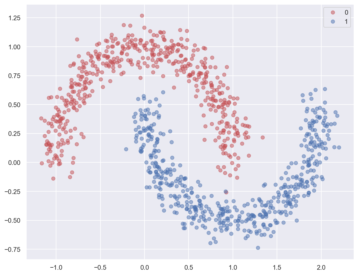
Example 1: training a dense network on planar data

# Generate moon-shaped, non-linearly separable data
x, y = make_moons(n_samples=1000, noise=0.10, random_state=0)

print(f'x: {x.shape}. y: {y.shape}')
plot_planar_data(x, y)

x: (1000, 2). y: (1000,)

# Create PyTorch tensors from Numpy data, with appropriate types
x_train = torch.from_numpy(x).float()
y_train = torch.from_numpy(y).long()

Model definition

# Use the nn package to define our model as a sequence of layers. nn.Sequential
# is a Module which contains other Modules, and applies them in sequence to
# produce its output. Each Linear Module computes output from input using a
# linear function, and holds internal Tensors for its weight and bias.
dense_model = nn.Sequential(
    nn.Linear(in_features=2, out_features=3),
    nn.Tanh(),
    nn.Linear(in_features=3, out_features=2)
)

print(dense_model)

Sequential(
  (0): Linear(in_features=2, out_features=3, bias=True)
  (1): Tanh()
  (2): Linear(in_features=3, out_features=2, bias=True)
)

# The nn package also contains definitions of popular loss functions; in this
# case we will use Cross Entropy as our loss function.
loss_fn = nn.CrossEntropyLoss()

# Used to enable training analysis through TensorBoard
# Writer will output to ./runs/ directory by default
writer = SummaryWriter()

Model training

learning_rate = 1.0
num_epochs = 2000

for epoch in range(num_epochs):
    # Forward pass: compute model prediction
    y_pred = dense_model(x_train)

    # Compute and print loss
    loss = loss_fn(y_pred, y_train)
    if epoch % 100 == 0:
        print(f"Epoch [{epoch+1:4}/{num_epochs}], loss: {loss:.6f}")
        # Write epoch loss for TensorBoard
        writer.add_scalar("Loss/train", loss.item(), epoch)

    # Zero the gradients before running the backward pass
    # Avoids accumulating gradients erroneously
    dense_model.zero_grad()

    # Backward pass: compute gradient of the loss w.r.t all the learnable parameters of the model
    loss.backward()

    # Update the weights using gradient descent
    # no_grad() avoids tracking operations history here
    with torch.no_grad():
        for param in dense_model.parameters():
            param -= learning_rate * param.grad


print(f"Training finished. Final loss: {loss:.6f}")

Epoch [   1/2000], loss: 0.615728
Epoch [ 101/2000], loss: 0.255993
Epoch [ 201/2000], loss: 0.254656
Epoch [ 301/2000], loss: 0.253930
Epoch [ 401/2000], loss: 0.253383
Epoch [ 501/2000], loss: 0.252850
Epoch [ 601/2000], loss: 0.252219
Epoch [ 701/2000], loss: 0.251364
Epoch [ 801/2000], loss: 0.250020
Epoch [ 901/2000], loss: 0.165510
Epoch [1001/2000], loss: 0.034935
Epoch [1101/2000], loss: 0.018792
Epoch [1201/2000], loss: 0.013152
Epoch [1301/2000], loss: 0.010341
Epoch [1401/2000], loss: 0.008661
Epoch [1501/2000], loss: 0.007542
Epoch [1601/2000], loss: 0.006741
Epoch [1701/2000], loss: 0.006137
Epoch [1801/2000], loss: 0.005665
Epoch [1901/2000], loss: 0.005284
Training finished. Final loss: 0.004974

Example 2: training a convnet on CIFAR10

Data loading and preparation

# Transform images of range [0, 1] into tensors of normalized range [-1, 1]
transform = transforms.Compose(
    [transforms.ToTensor(),
     transforms.Normalize((0.5, 0.5, 0.5), (0.5, 0.5, 0.5))])

# Load training set
trainset = torchvision.datasets.CIFAR10(
    root="./data", train=True, download=True, transform=transform
)
# Get an iterable from training set
trainloader = torch.utils.data.DataLoader(
    trainset, batch_size=4, shuffle=True, num_workers=2
)

testset = torchvision.datasets.CIFAR10(
    root="./data", train=False, download=True, transform=transform
)
testloader = torch.utils.data.DataLoader(
    testset, batch_size=4, shuffle=False, num_workers=2
)

Files already downloaded and verified
Files already downloaded and verified

Expected network architecture

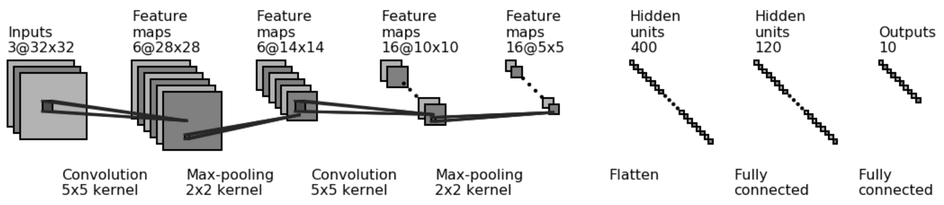
# Define a CNN that takes (3, 32, 32) tensors as input (channel-first)
class Net(nn.Module):
    def __init__(self):
        super(Net, self).__init__()
        self.conv1 = nn.Conv2d(in_channels=3, out_channels=6, kernel_size=5)
        self.pool = nn.MaxPool2d(kernel_size=2, stride=2)
        self.conv2 = nn.Conv2d(in_channels=6, out_channels=16, kernel_size=5)
        # Convolution output is 16 5x5 feature maps, flattened as a 400 elements vectors
        self.fc1 = nn.Linear(in_features=16 * 5 * 5, out_features=120)
        self.fc2 = nn.Linear(in_features=120, out_features=10)

    def forward(self, x):
        x = self.pool(F.relu(self.conv1(x)))
        x = self.pool(F.relu(self.conv2(x)))
        x = x.view(-1, 16 * 5 * 5)
        x = F.relu(self.fc1(x))
        x = self.fc2(x)
        return x

cnn_model = Net()
print(cnn_model)

Net(
  (conv1): Conv2d(3, 6, kernel_size=(5, 5), stride=(1, 1))
  (pool): MaxPool2d(kernel_size=2, stride=2, padding=0, dilation=1, ceil_mode=False)
  (conv2): Conv2d(6, 16, kernel_size=(5, 5), stride=(1, 1))
  (fc1): Linear(in_features=400, out_features=120, bias=True)
  (fc2): Linear(in_features=120, out_features=10, bias=True)
)

Model training

criterion = nn.CrossEntropyLoss()
optimizer = optim.SGD(cnn_model.parameters(), lr=0.001, momentum=0.9)

num_epochs = 2

# Loop over the dataset multiple times
for epoch in range(num_epochs):
    running_loss = 0.0

    for i, data in enumerate(trainloader, 0):
        # Get the inputs; data is a list of [inputs, labels]
        # inputs is a 4D tensor of shape (batch size, channels, rows, cols)
        # labels is a 1D tensor of shape (batch size,)
        inputs, labels = data

        # Reset the parameter gradients
        optimizer.zero_grad()

        # Forward pass
        outputs = cnn_model(inputs)

        # Loos computation
        loss = criterion(outputs, labels)

        # Backward pass
        loss.backward()

        # GD step
        optimizer.step()

        # Print statistics
        running_loss += loss.item()
        if i % 2000 == 1999:  # print every 2000 mini-batches
            print(
                f"Epoch [{epoch+1}/{num_epochs}], batch {i+1:5}, loss: {running_loss / 2000:.6f}"
            )
            running_loss = 0.0


print(f"Training finished")

Epoch [1/2], batch  2000, loss: 2.108662
Epoch [1/2], batch  4000, loss: 1.737864
Epoch [1/2], batch  6000, loss: 1.592003
Epoch [1/2], batch  8000, loss: 1.507958
Epoch [1/2], batch 10000, loss: 1.445331
Epoch [1/2], batch 12000, loss: 1.393309
Epoch [2/2], batch  2000, loss: 1.327055
Epoch [2/2], batch  4000, loss: 1.302520
Epoch [2/2], batch  6000, loss: 1.286105
Epoch [2/2], batch  8000, loss: 1.265079
Epoch [2/2], batch 10000, loss: 1.240521
Epoch [2/2], batch 12000, loss: 1.270833
Training finished

Model evaluation

correct = 0
total = 0

with torch.no_grad():
    for data in testloader:
        # Load inputs and labels
        images, labels = data
        # Compute model predictions for batch. Shape is (batch size, number of classes) so(4, 10) here
        outputs = cnn_model(images)
        # Get the indexes of maximum values along the second axis
        # This gives us the predicted classes (those with the highest prediction value)
        _, predicted = torch.max(outputs.data, dim=1)
        total += labels.size(0)
        # Add the number of correct predictions for the batch to the total count
        correct += (predicted == labels).sum().item()

print(f"Test acccuracy: {(100 * correct / total)}%")

Test acccuracy: 56.16%

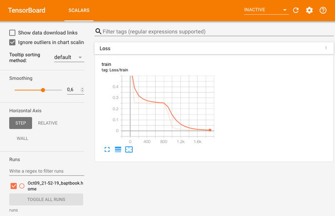
Training analysis with TensorBoard

More info on PyTorch/TensorBoard integration here.